Holonomic Odometry Testbed

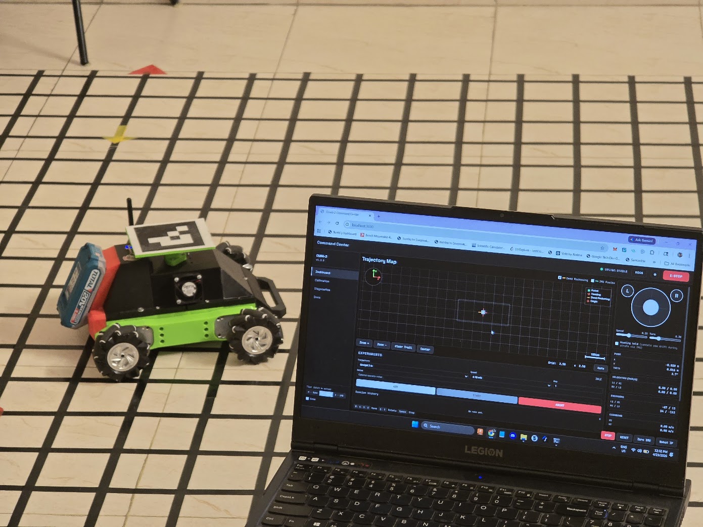
I chose mecanum wheels for this project mostly because the math behind them is worth working through properly. A mecanum robot can translate in any direction without rotating first — strafe sideways, move diagonally, spin on the spot — and all of it falls out of a single kinematic model derived from first principles. That model is elegant. Implementing it on real hardware, and then trying to localise accurately with it, is where it gets interesting.

The core problem is that mecanum wheels are sliding contacts, not pure rolling ones. Each wheel carries angled passive rollers along its rim; motion in any direction involves some roller scuff, and that scuff is not in the model. It accumulates into heading drift and position error over a run. Real platforms deal with this through laser range-finders, external cameras, or UWB anchors. The goal here was to understand the problem from the ground up: derive the kinematics by hand, build a testbed to run them on, and then layer feedback — per-wheel PID, then IMU fusion — to see how much of that error each layer can cancel. The platform and all its software are open-source as open-omnibot.

Building the platform

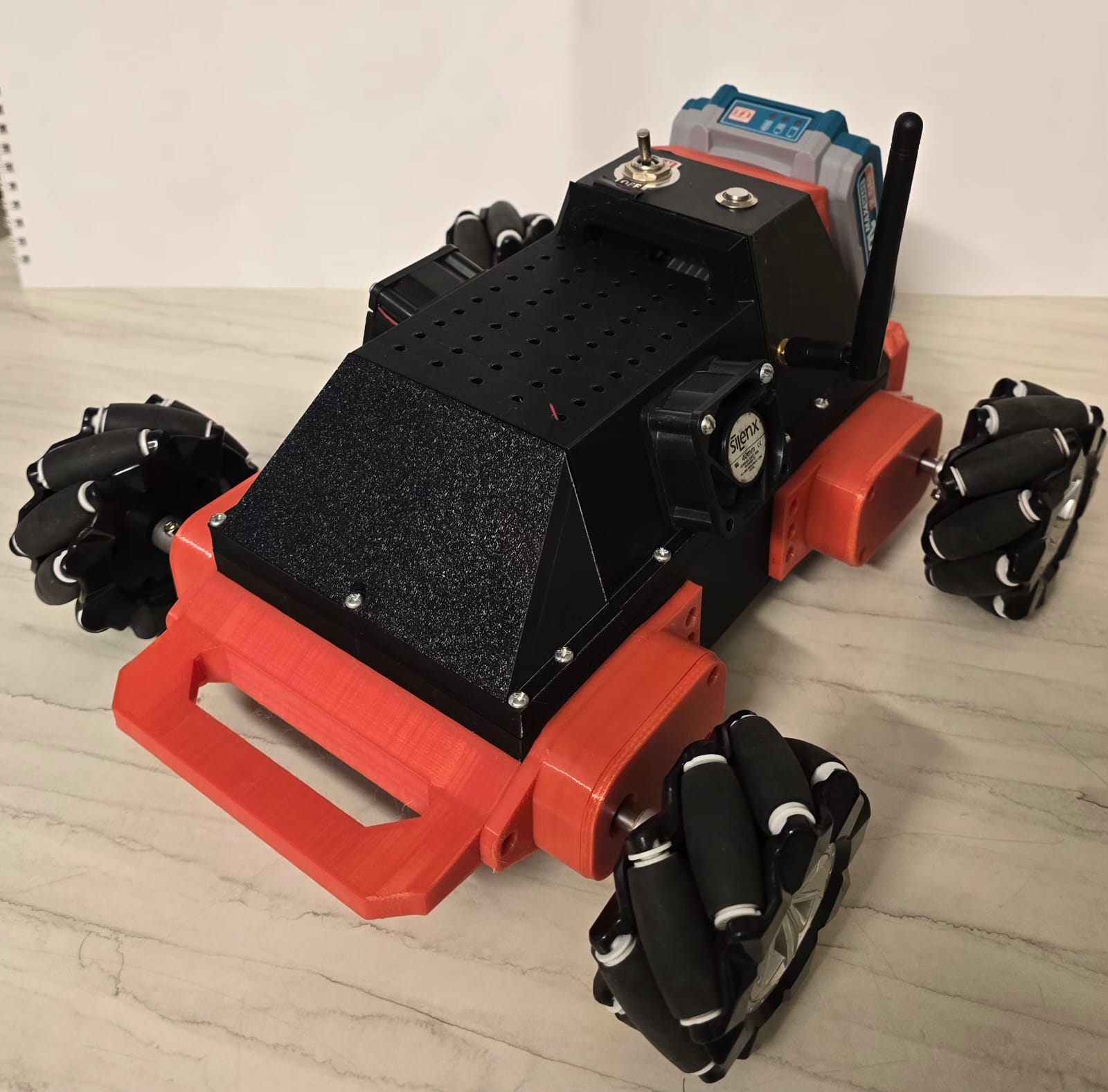
The chassis is a 3D-printed PETG frame carrying four 80 mm-diameter mecanum wheels in the standard X-configuration: left-side rollers at +45° and right-side rollers at −45°. Each wheel is driven by an independent DCGM-3865 brushed DC gearmotor with a 42:1 gear reduction. The motors carry 13-pulse-per-revolution quadrature encoders on the motor shaft; after the gearbox and 2× edge counting on one channel, this yields 1092 counts per wheel revolution — about 0.23 mm per count of linear resolution.

The chassis went through several iterations; the final version has adjustable motor-mount heights to level the wheel contact plane after assembly, compensating for variance in 3D-print dimensional accuracy.

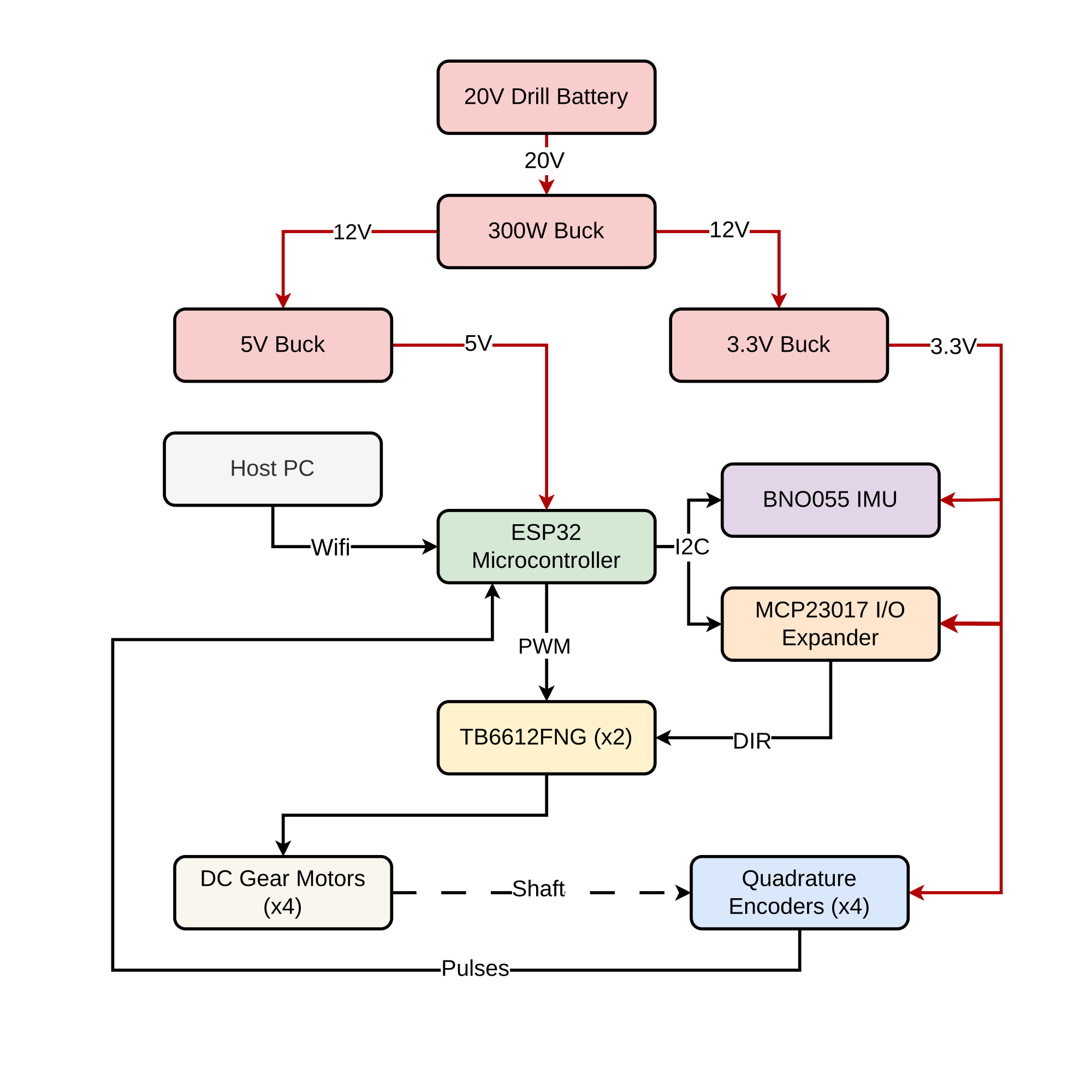
Power. The power system is a commercial 20 V cordless-drill battery on a custom 3D-printed mount — overbuilt for the load, field-replaceable, and protected by an integrated BMS. A 300 W buck converter regulates to 12 V for the motors; two downstream converters derive 5 V for the ESP32 and 3.3 V for the IMU and encoder logic.

Electronics. Motor control is handled by two TB6612FNG dual H-bridge modules, one per motor pair. The ESP32 generates PWM on its LEDC peripheral at 1 kHz with 8-bit resolution. Direction lines for the eight motor channels are driven through an MCP23017 16-bit I²C GPIO expander rather than directly from ESP32 pins — this was a deliberate choice to reserve the interrupt-capable GPIO pins for the encoder channels, which need two pins each. The I²C direction writes happen only when a motor’s direction actually changes, roughly once per second, so the bandwidth penalty is negligible.

Sensing. The BNO055 IMU sits on a dedicated 3D-printed bracket fastened to the geometric centre of the chassis — underneath, between the four wheel footprints. Placing it there keeps the IMU coincident with the instantaneous centre of rotation under pure-yaw commands, minimising the centripetal acceleration it sees during turns. The firmware runs the BNO055 in IMUPLUS mode (accelerometer + gyroscope fusion, no magnetometer).

The kinematics

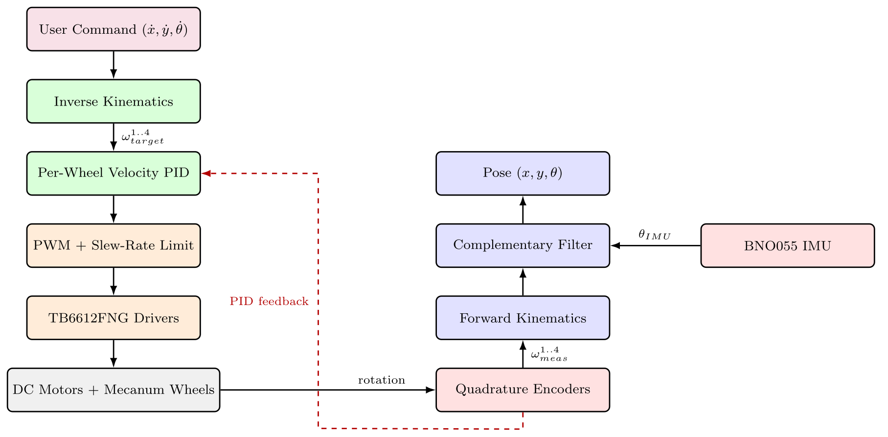
Working through the kinematics from first principles is the core of what this project is about. The kinematic model connects the four wheel angular velocities ω₁…ω₄ to the body-frame planar velocity (ẋ, ẏ, θ̇). Two maps come out of it: the inverse kinematics (body velocity → wheel speeds, what the trajectory executor needs every 50 Hz) and the forward kinematics (wheel speeds → body velocity, what the odometry integrator uses to track pose).

Coordinate frames

Two right-handed frames are used throughout. The world frame {W} is fixed to the lab floor with axes X_W and Y_W. The body frame {B} is attached to the robot centre, with X_B pointing forward and Y_B pointing left. The robot’s planar pose is the state vector:

where (x, y) is the body-frame origin in the world frame and θ is the heading angle measured counter-clockwise from X_W. The rotation from body to world is the standard 2D rotation matrix:

R(θ) is used later in the pose integration step to rotate body-frame velocities into world-frame displacements.

Geometry and wheel layout

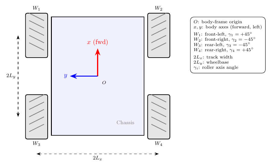
Wheels are indexed front-left (1), front-right (2), rear-left (3), rear-right (4). Each wheel has radius r = 40 mm. The four wheel-centre positions in the body frame are:

where half-track width Lₓ = 117.5 mm and half-wheelbase Lᵧ = 95.3 mm. The mecanum roller axes make ±45° with the wheel axle; diagonal pairs {W₁, W₄} and {W₂, W₃} share the same roller angle:

Wheel constraint equation

Each mecanum wheel has two independent slip axes: the wheel rolls actively about its axle (driven by the motor), and the roller at the ground contact rolls passively along its own axis. The no-slip constraint applies only in the direction perpendicular to the roller axis; along the roller axis the wheel slides freely.

The body-frame linear velocity of wheel i’s centre follows from rigid-body kinematics:

The unit vector perpendicular to roller i’s axis, in the body frame, is n̂ᵢ = (cos γᵢ, −sin γᵢ). The wheel rim translates the contact point at speed r·ωᵢ along the body X-axis. Matching the n̂ᵢ component of rim velocity to the n̂ᵢ component of wheel-centre velocity gives:

For γᵢ = ±45°, cos γᵢ = 1/√2 and sin γᵢ = ±1/√2. Dividing through by cos γᵢ and substituting tan γᵢ = ±1:

This is the per-wheel constraint equation. Everything else — IK and FK — is just this equation applied four times.

Inverse kinematics

Substituting each wheel’s position (xᵢ, yᵢ) and roller angle γᵢ into the constraint, and letting L ≡ Lₓ + Lᵧ:

Stacking into matrix form:

This matrix J_IK maps commanded body velocity to target wheel speeds. Verification by pure motions:

• Pure forward (ẋ > 0, ẏ = θ̇ = 0): all four wheels spin forward at ωᵢ = ẋ/r.
• Pure left strafe (ẏ > 0, ẋ = θ̇ = 0): ω₁, ω₄ < 0 and ω₂, ω₃ > 0 — the characteristic X-pattern that generates lateral force.
• Pure CCW rotation (θ̇ > 0, ẋ = ẏ = 0): ω₁, ω₃ < 0 (left wheels back) and ω₂, ω₄ > 0 (right wheels forward).

Forward kinematics via pseudo-inverse

J_IK is 4×3 — more equations than unknowns — so no exact inverse exists. The Moore-Penrose pseudo-inverse gives the least-squares body velocity consistent with the four measured wheel speeds:

Computing J_IKᵀ J_IK explicitly:

This is diagonal because the wheel positions and roller geometry are symmetric about both body-frame axes. The inverse is immediate:

Combining gives the full pseudo-inverse:

Substituting back:

Physical reading: forward velocity is the mean of all four wheels; lateral velocity is the differential between diagonal pairs {ω₂, ω₃} and {ω₁, ω₄}; angular velocity is the right-minus-left differential scaled by 1/L.

The pseudo-inverse also reveals where the model breaks down. J_IKᵀ has a null space — wheel-speed combinations that look like zero body motion but correspond to roller slip. A mecanum wheel scuffs its rollers any time the contact force has a component along the roller axis; that scuff never registers in encoder counts, so it is invisible to the forward kinematics. Over time the pose integrator accumulates that invisible error into heading drift and lateral offset. This is structural, not a bug; encoder odometry on a mecanum platform will always drift.

World-frame pose integration

The forward kinematics returns body-frame velocities. To track world-frame pose, these are rotated by the current heading using R(θ) and integrated:

The cross-coupling between (ẋ, ẏ) and θ makes this a nonlinear system — which is exactly why the EKF is the natural estimator when external reference measurements are added later.

Euler vs midpoint integration. The simplest discrete update is Euler:

Euler is first-order accurate and introduces systematic error during rotation because the heading is held constant across the step. Midpoint integration corrects this by evaluating the rotation at the half-step:

This is second-order accurate. The firmware runs midpoint integration at Δt = 20 ms, trading a negligible per-step cost for improved accuracy on rotation-rich trajectories.

Encoder velocity estimation

The wheel angular velocities ωᵢ used in the forward kinematics are reconstructed from quadrature-encoder count deltas. Given count change Δnᵢ over interval Δt, and N = 1092 counts per wheel revolution:

Linear wheel-rim velocity follows as vᵢ = r·ωᵢ. For this platform with r = 40 mm and N = 1092, the per-count linear resolution is:

This resolution is several orders of magnitude finer than the closure errors measured in experiments, so encoder quantisation contributes negligibly to the odometry error budget.

Error sources

Residual errors that accumulate in Tier 1 encoder odometry fall into two categories:

Systematic errors — inaccuracies in r, Lₓ, Lᵧ, or the nominal ±45° roller angles — bias the odometry in a repeatable way and can in principle be reduced by calibration.

Non-systematic errors — mecanum roller slip (especially during lateral motion), surface irregularities, load variations, and per-motor velocity spread — are stochastic and bounded from below by the physics of the platform rather than the model. Both classes accumulate unboundedly during open-loop integration: position error grows linearly with distance travelled, and heading error causes position error to grow quadratically over time. No purely proprioceptive scheme can hold long-horizon accuracy without an external reference or an independent heading measurement. IMU fusion (Tier 2) and a future UWB-anchored tier are the two routes for bounding this drift.

The firmware

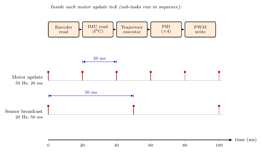
The ESP32 runs a single-threaded Arduino loop at approximately 1 kHz with two fixed-interval triggers:

• 50 Hz motor-update tick: reads encoders, reads IMU, runs the trajectory executor, runs per-wheel PID, writes PWM.
• 20 Hz sensor-broadcast tick: assembles and sends a JSON snapshot of all sensor state over WebSocket to the host computer.

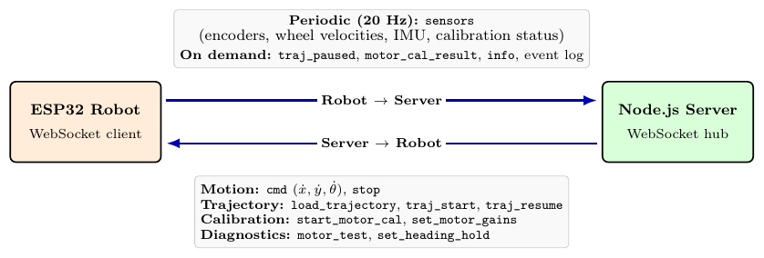
WebSocket protocol. All robot–server communication is a single bidirectional JSON channel. The robot broadcasts a sensors message at 20 Hz containing encoder counts, wheel velocities, IMU state, and calibration status. The server sends motion commands (cmd), trajectory control messages (load_trajectory, traj_start, traj_resume), and calibration and diagnostic commands. A 500 ms command-timeout on the firmware side stops the robot if the server drops off the network.

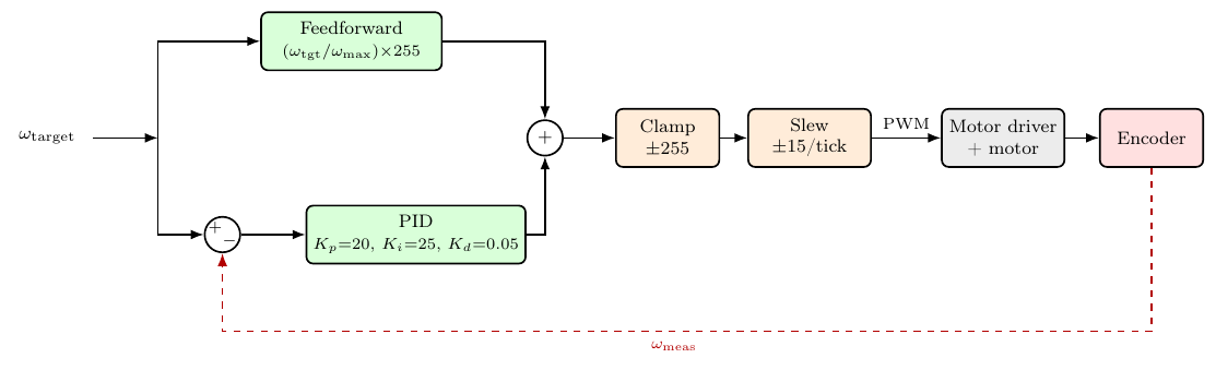
Per-wheel velocity PID. Each of the four wheels has an independent velocity PID loop with a calibrated feedforward term. At each 50 Hz tick, the inverse kinematics maps the commanded body velocity to four target wheel speeds; a feedforward PWM is computed linearly from the target speed; the PID correction handles the residual between target and measured. The gains were tuned empirically on the bench: K_p = 20, K_i = 25, K_d = 0.05. The integrator is clamped to ±200 PWM units and only reset on explicit events (safety stop, pause–resume, new trajectory load), so the control loop benefits from the bias it learned during previous segments.

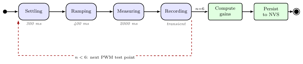
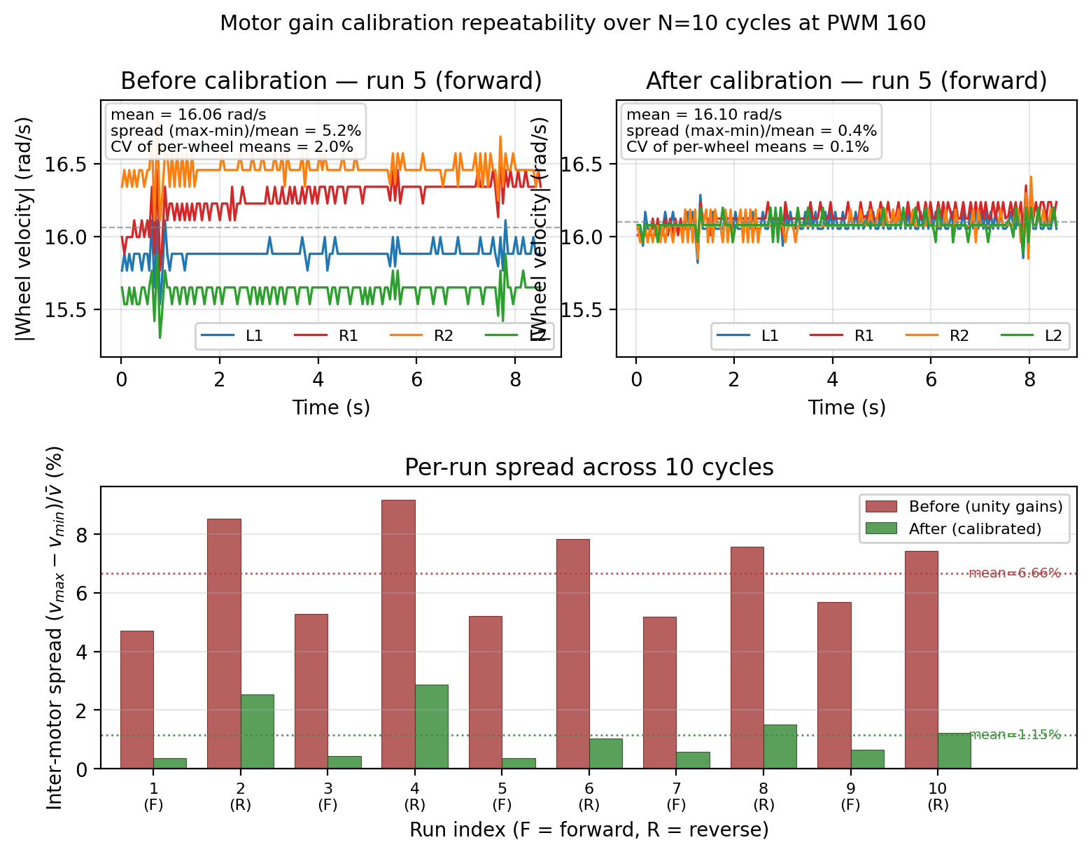
Motor calibration. Per-motor manufacturing variance — brush contact, gearbox backlash, winding resistance — produces different wheel velocities at the same applied PWM. On a mecanum platform this projects directly into body-frame yaw or strafe bias. An automated calibration routine sweeps six PWM test points (±100, ±160, ±220), measures encoder counts at each, and computes per-motor per-direction gain factors that bring all four motors to the group mean. Gains are stored in ESP32 non-volatile memory and reloaded on every boot. Critically, the gain is applied on the commanded PWM side, not the measurement side — the motor physically receives a corrected PWM and the encoders honestly report what the wheel is actually doing.

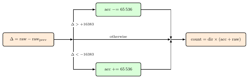
Encoder overflow. The ESP32 PCNT peripheral maintains a signed 16-bit counter per encoder channel. At 1092 counts per revolution, this overflows every 30 wheel revolutions — about 3.8 m of forward travel at typical speeds. The firmware detects wraps by checking whether consecutive inter-tick deltas exceed half the counter range (a physically impossible jump), and applies a ±65,536 correction to a running overflow accumulator. This logic is covered by unit tests that exercise zero-crossing, threshold-boundary, and direction-inversion cases.

Three tiers of error correction. Three localization modes are implemented on the same hardware, each adding one layer of compensation for the structural slip the kinematics cannot model:

• Tier 0 (open-loop): fixed-PWM lookup table per cardinal direction. No sensor feedback, no pose estimation. Timer-based segment execution only. This is the baseline — pure kinematics with no correction, so all roller slip and motor variance accumulates unchecked.
• Tier 1 (encoder odometry): per-wheel velocity PID closes the loop on wheel speed; the mecanum forward kinematics then integrates encoder deltas into (x, y, θ) using midpoint integration. This corrects for PWM-to-velocity nonlinearity and motor variance, but roller slip is still invisible to the encoders, so heading drift remains.
• Tier 2 (complementary filter): same as Tier 1 for position, but heading is fused: θ_fused = (1 − α)·θ_odom + α·(θ_IMU − θ_offset) with α = 0.98. The IMU has 98% authority over heading, which is the component most corrupted by slip; a heading-hold proportional controller also engages on translation segments to actively suppress uncommanded yaw.

EKF or UKF fusion alongside an external reference — UWB anchors or an overhead camera — is the natural next step for closing the gap that roller scuff leaves open.

The dashboard and pipeline

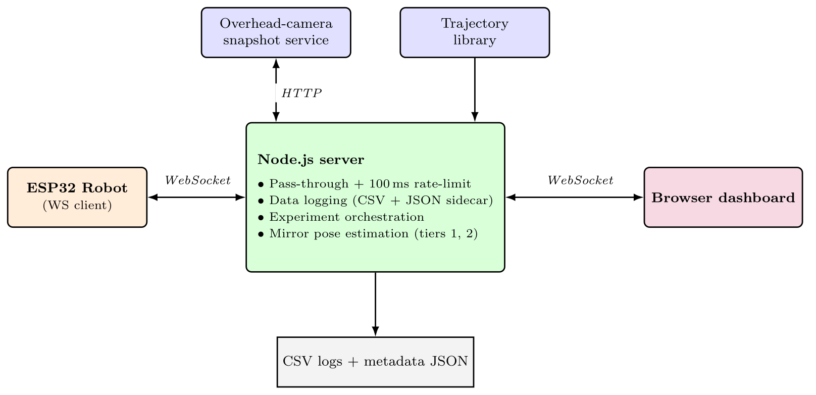
A Node.js server on the host laptop bridges robot WebSocket frames to the browser dashboard, logs every run to CSV, and orchestrates the ground-truth capture workflow. The browser dashboard handles manual driving, motor calibration, preflight diagnostics, experiment execution, and in-app documentation — all without a separate toolchain; any browser on the local Wi-Fi can drive the robot.

Every run is logged to CSV at 20 Hz. After a campaign, an offline-replay pipeline re-derives the same pose estimates deterministically from the raw log, so a new estimator can be benchmarked against the full historical dataset without re-running the robot.

Status

Thesis defended and graded, Spring 2026. The platform, firmware, server, browser dashboard, and offline analysis pipeline are open-source at samiul-hoque/open-omnibot as a testbed for evaluating sensor-fusion and localization algorithms on four-wheeled holonomic robots.

A video walkthrough of the kinematics — inverse kinematics, forward kinematics, and the slip problem — is in progress. It will be linked here when it is up.

Earlier work on the same chassis family

A small earlier RC-controlled pick-and-place build on a mecanum-wheel chassis was written up by classmates and published at ICIPRoB 2024 (see Omnidirectional Pick-and-Place Robot — ICIPRoB 2024). The thesis platform is a distinct build with a different controller, sensors, and firmware — but it sits in the same line of work on mecanum-wheel holonomic robots at IUB.